Analysis of seabird data from the open sea

We use statistical analyses of count data to quantify the expected occurrence of seabirds in all-encompassing areas. First, we analyse the relationship between seabird occurrence and diverse geographical variables. This relationship is then used to calculate the expected, or predicted, seabird occurrence in all-encompassing areas. Here, we present a detailed description of the methodology we have used.

Statistical modelling

The transect data only cover thin strips of the large sea areas where it is desirable to predict the distribution of the seabirds. As a result of the birds’ flock formations, the data contains large local variations in density. To the extent that this variation cannot be explained by specific geographical areas, it is desirable to remove it from the predictions. To remove this kind of random local variation, and in order to predict densities in all-encompassing areas, including areas with little data, the data was modelled with geographically fixed explanatory variables in two-step models. The models were then used to predict the density of the different species in a grid where the explanatory variables were known.

The analyses were run separately for all species, seasons and sea areas. In the analyses of a given sea area, data was included from 200 km into adjacent sea areas, in order to better the estimates for the boundaries between sea areas.

Data aggregration

Before the data was modelled, they were combined according to a spatial scale appropriate to the total area being analysed. The purpose of this type of aggregation is to adjust the observational scale to the geographical pattern one wishes to predict. The influence of pseudo replication is thereby reduced, the sample size becomes more manageable, and random local variation is smoothed out.

We chose to use an observational scale of 50 km. It was complicated to aggregate the data in a systematic way, as a result of the frequent interruptions in the observations and change in transect direction. We chose a procedure where the aggregation occurred successively and chronologically along the completed transects. An observation was included in an aggregated point if the distance from the point to the midpoint in the aggregated point was less than 25 km, and if the time difference between the point and the average in the aggregated point was less than 6 hours. As a result of the methodology, the transect length varied between the aggregated points, and transect length was therefore corrected for in the analyses. Aggregated points where the transect length was less than 5 km were excluded from the selection.

**A flock of common guillemots.** As seabirds gather in large and transient flocks they are particularly vulnerable to spatially limited disturbances such as oil spills, or ending up as bycatch in fishing gear. Even if the scope of damage is potentially large, there will be large uncertainty as to whether a given disturbance will overlap spatially and temporally with a gathering of seabirds. This means that a given disturbance in certain instances can affect many birds, while the same disturbance in many other instances will have little effect. Important questions for seabird studies on the open sea have therefore been: How predictable are these types of seabird gatherings? To what degree can we make detailed maps of seabird distributions? To answer the first question, repeated measurements are needed over a longer time period. To answer the second question, good geographical coverage of the measurements is needed, as well as statistical methods that handle highly aggregated distributions and large datasets. Photo: Per Fauchald

Two-step analyses

Pelagic organisms, including seabirds, have a clumped spatial distribution. In practice, this means that spatial data of this type of organism contains many observations where no individuals have been counted (null observations), and some observations where many individuals have been counted. Due to the many null observations, this type of data is called zero-inflated data. Two-step modelling is an effective way to handle this kind of data.

The purpose of the models is to estimate the relationship between observed density of seabirds and geographically-fixed explanatory variables, in order to use these estimates to predict density in all-encompassing areas where the explanatory variables are known.

The first step in the two-step analyses was to model the presence/absence of birds. In this step a binomial distribution with “logit link” function was used. In step 2 we modelled the number of birds in the observations where birds were actually present. In this step a Gamma distribution with “log link” function was used. Ideally at this stage a truncated Poisson or a truncated negative binomial distribution would have been used. However, these models would not converge, most likely since a number of the observations had very high values; nevertheless, the Gamma models worked adequately as an approach.

In order to model the relationships with the geographically fixed explanatory variables, non-linear Generalized Additive Models (GAM) were used from the “mgcv” library package in R v.2.10.1 (R Development Core team, 2009). The explanatory variables were the x and y directions (respectively, west-east and south-north), depth (d) and distance to coast (c). Geographic position was modelled with a two-dimensional smoothing function: g(x,y). d and c were modelled with one-dimensional smoothing functions: s(·). “Tensor product” smoothing with cubic regression splints was used as a basis. Optimal smoothing was defined as Generalized Cross Validation (GCV).

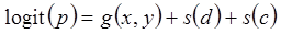
In the first step, the probability of bird presence was modelled with “logit link” and binomial distribution:

In the second step, the number of birds was modelled for the observations where the number of birds was greater than zero, with “log_e link” and Gamma distribution:

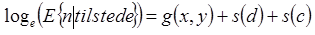
where E is expectation. Distance travelled (log_e-transformed) for each observation was used as an “offset” in the models.

Model predictions

Based on the estimates in the models, the “predict” function in the “mgcv” library package was used to predict the expected geographical distribution of birds in a 10×10 km² grid that covers the study area every season. The predicted probability of bird presence in a given cell was found with the help of the binomial model. In the same way, the predicted number of birds in a given cell was found with the Gamma model. The expected number of birds in a given cell is thus given by:

Uncertainty: Bootstrap analyses

Uncertainty in the estimates will depend upon the degree of coverage (sample size) and variation in distribution, for each respective species. The uncertainty in the predictions is not easily calculated, and we therefore chose to conduct bootstrap analyses to find standard errors and confidence intervals for the predictions in relation to geographic distribution and annual abundance in the Barents Sea.

The analyses described above were conducted for 2000 bootstrap selections (random sampling of the dataset with replacement). The estimates from the bootstrap selections were log-normal distributed, and the standard error was calculated for each log₁₀-transformed value. The 95% confidence interval was calculated from the selection.

When calculating uncertainty in relation to annual abundance, the bootstrap selection reflects both uncertainty with regards to differences between years, as well as uncertainty with regards to the average abundance in the study area (the intercept). For species with distributions at the boundaries of the study area, the uncertainty in the intercept was relatively large. The intercept was therefore standardised the same as the average abundance (over all years) from the analysis of the original selection. The confidence interval and standard error therefore represent uncertainty with regards to differences between years, not uncertainty with regards to average abundance.